Catenary Derivation - more detail

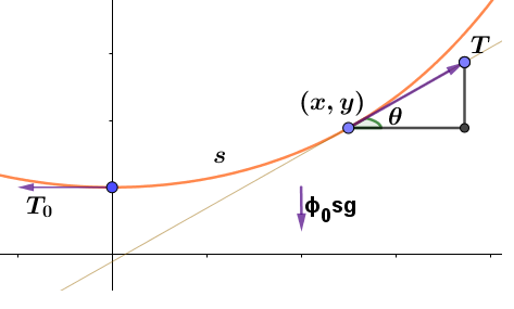
Equilibrium is achieved by the three forces, tension in the direction of $T,$ tension in the direction of $T_{0},$ and gravity, expressed as $\phi_{0}sg,$ See figure 1. From trigonometry, we find, $$T_{0}=T\cos\theta \tag{1} \label{1}$$ $$\phi_{0}sg=T\sin\theta \tag{2} \label{2}$$ and $$\tan\theta=\frac{T\sin\theta}{T\cos\theta}=\frac{\sin\theta}{\cos\theta}=\frac{\phi_{0}sg}{T_{0}} \tag{3} \label{3}$$

Traditionally, a constant, $a$, is defined as $$a=\frac{T_{0}}{\phi_{0}g}, \tag{4} \label{4}$$ and from $\eqref{3}$ $$tan\,\theta=\frac{s}{a}.$$ A unit analysis shows that $\tan\,\theta$ is unit-less, as it must be, and that $a$ has units of meters. $$\text{Unit Analysis: }a=\frac{T_{0}}{\phi_{0}g}=\frac{\frac{kg\cdot m}{s^{2}}}{\left(\frac{kg}{m}\right)\cdot\left(\frac{m}{s^{2}}\right)}=m$$ We can remember that $\tan\,\theta=slope=dy/dx$ and make that substitution. $$\frac{s}{a}=\frac{dy}{dx}=y'=\tan\theta. \tag{5} \label{5}$$ We can also look back at Standard Arc Length to see that arc length, $s$ is $$s=\int_{a}^{b}\sqrt{1+\left(\frac{dy}{dx}\right)^{2}}\,dx$$ and substituting the integral for $s$ into equation $\eqref{5}$, $$\frac{1}{a}\int_{a}^{b}\sqrt{1+\left(\frac{dy}{dx}\right)^{2}}\,dx=\frac{dy}{dx}.$$ In this case the integrations limits are $0$ to $x.$ We can differentiate both sides to remove the integral leaving a second order differential equation. $$\frac{1}{a}\sqrt{1+\left(\frac{dy}{dx}\right)^{2}}=\frac{d^{2}y}{dx^{2}}$$ This could get rather involved to solve but we can give it try. Let $p=dy/dx$ and change the problem to a first order ODE. $$\frac{1}{a}\sqrt{1+p^{2}}=\frac{dp}{dx}$$ Separate the variables. $$\frac{dx}{a}=\frac{1}{\left(1+p^{2}\right)^{1/2}}dp$$ The right side is a standard integral, although not one that is very common. It can be worked through with multiple $u$ substitutions. However, Standard Mathematical Tables 27th edition from CRC Press gives this integral: $$\text{Integral \#157: }\intop\frac{dx}{\sqrt{x^{2}\pm\mathrm{a}^{2}}}=ln\left(x+\sqrt{x^{2}\pm\mathrm{a}^{2}}\right)$$ Using that result, $$\frac{1}{a}\intop dx=\intop\frac{1}{\sqrt{1+p^{2}}}dp$$ $$\frac{1}{a}x=ln\left(p+\sqrt{1+p^{2}}\right)+const$$

Aside: Where we are going with this is to two equations given below as $\eqref{7}$ and $\eqref{11}$. These will be the two equations that we rely on to solve problems. Some sources that report to show this derivation skip over the calculus and algebra that we will go through next and just miraculously show the two equations. In fact, some do not even show the first one and it just suddenly appears when solving problems.

From the figure we can see that when $x=0$ that $dy/dx=0$ and remembering that $p=dy/dx$ we can solve for the const. $$\frac{1}{a}\cdot0=ln\left(0+\sqrt{1+0^{2}}\right)+const$$ $$-const=ln(1)=0\rightarrow const=0.$$ Therefore $$\frac{1}{a}x=ln\left(\sqrt{1+p^{2}}+p\right)$$ So now for some algebra.

Raise both sides the the power e. $$e^{\frac{x}{a}}=\sqrt{1+p^{2}}+p$$ Subtract $p$ from both sides. $$e^{\frac{x}{a}}-p=\sqrt{1+p^{2}}$$ Square both sides. $$\left(e^{\frac{x}{a}}\right)^{2}-2pe^{\frac{x}{a}}+p^{2}=1+p^{2}$$ Cancel out $p^{2}.$ $$\left(e^{\frac{x}{a}}\right)^{2}-2pe^{\frac{x}{a}}=1$$ Solve for variable $p.$ $$p=\frac{1-\left(e^{\frac{x}{a}}\right)^{2}}{-2e^{\frac{x}{a}}}=\frac{\left(e^{\frac{x}{a}}\right)^{2}-1}{2e^{\frac{x}{a}}}$$ Separate the terms. $$p=\frac{\left(e^{\frac{x}{a}}\right)^{2}}{2e^{\frac{x}{a}}}-\frac{1}{2e^{\frac{x}{a}}}$$ Cancel $e^{\frac{x}{a}}$ from the left term and elevate $e^{\frac{x}{a}}$ into the numerator in the right term. $$p=\frac{dy}{dx}=\frac{e^{\frac{x}{a}}}{2}-\frac{e^{-\frac{x}{a}}}{2}=\frac{e^{\frac{x}{a}}-e^{-\frac{x}{a}}}{2} \tag{6} \label{6}$$

Since $p=dy/dx=y'=s/a$ (from $\eqref{5}$) and using $\sinh(x)=\mathbf{\frac{e^{x}-e^{-x}}{2}}$ we get an important side benefit that $$\frac{s}{a}=\sinh\left(\frac{x}{a}\right). \tag{7} \label{7}$$

To get $y$ replace $p$ with $dy/dx.$ We can again separate variables and integrate both sides. $$\intop dy=\intop\frac{e^{\frac{x}{a}}}{2}dx-\intop\frac{e^{-\frac{x}{a}}}{2}dx \tag{8} \label{8}$$ The easiest way to do this integral is to combine the terms and use the Euler identity (see below). $$\intop dy=\int\left(\frac{e^{\frac{x}{a}}}{2}-\frac{e^{-\frac{x}{a}}}{2}\right)dx=\int\sinh\left(\frac{x}{a}\right)dx$$ Now substitute $u=\frac{x}{a}$ so $du/dx=1/a$ and $dx=a\cdot du.$ $$\intop dy=\int\sinh\left(u\right)a\cdot du=a\int\sinh(u)du$$ Again, we look up this integral. $\int\sinh(u)du=\cosh(u)$ and replace $u$ with $x/a.$ $$y=a\cosh\left(\frac{x}{a}\right) \tag{9} \label{9}$$ Alternatively, we integrate all three terms of $\eqref{8}$, factor and use Euler to get the same result done pretty much the same way. $$y=\frac{a}{2}e^{\frac{x}{a}}+\frac{a}{2}e^{-\frac{x}{a}} \tag{10} \label{10}$$ From Euler, we have the identities: $$\sinh(x)=\frac{e^{x}-e^{-x}}{2}\qquad\text{and}\qquad\cosh(x)=\frac{e^{x}+e^{-x}}{2}$$

Equation $\eqref{10}$ can be used to make figure 1. However, if we look at the Euler equations, we will see that $\eqref{10}$ can be expressed as $$y=a\cdot cosh(\frac{x}{a}) \tag{11} \label{11}$$ which is why we introduced the Euler formula in a prior section. For solving catenary problems, it is important to notice that when $x=0$ then $y=a.$ Therefore, if the problem is arranged to assure that $x=0$ is the bottom of the catenary, then $a$ will be the distance from the origin ($x$-axis) to the lowest point of sag. Finally, and most important. The $x$-axis in catenary problems usually isn't the ground! We will do a couple of examples, as this is really not obvious. Also, these are often easier to solve numerically than analytically.